Q-learning: From Pavlov’s Experiments to Modern Neurorehabilitation

Q-learning (Q learning in Spanish) has evolved considerably since the early behavioral experiments such as Pavlovian classical conditioning, becoming one of the most important techniques in the field of Machine Learning. Below, we will explore how it has developed and its application in neurorrehabilitation and cognitive stimulation.

Pavlov’s experiments

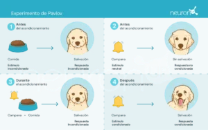
Ivan Pavlov, a Russian physiologist from the late 19th century, is recognized for establishing the foundations of behavioral psychology through his experiments on classical conditioning. In these experiments, Pavlov showed that dogs could learn to associate a neutral stimulus, such as the sound of a bell, with an unconditioned stimulus, like food, thus eliciting an unconditioned response: salivation.

This experiment was fundamental to demonstrate that behavior can be acquired by association, a crucial concept that later influenced the development of reinforcement learning theories. 

Reinforcement learning theories

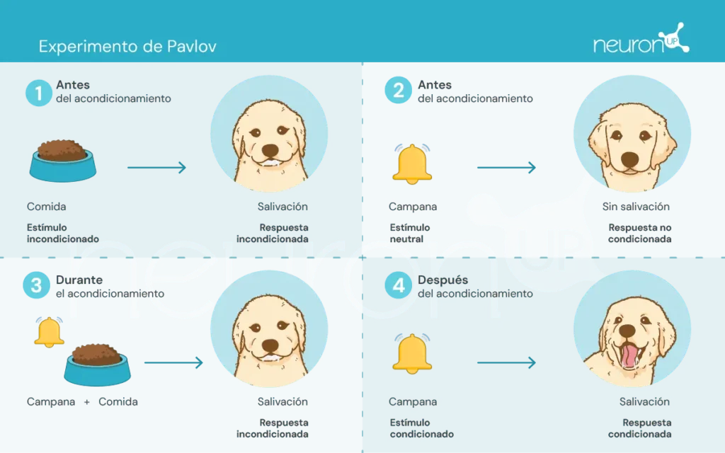
These theories focus on how humans and animals learn behaviors from the consequences of their actions, which has been essential for the design of algorithms such as Q-learning.

There are some key concepts we should become familiar with before continuing:

• Agent: responsible for performing the action.
• Environment: the surroundings where the agent moves and interacts. 
• State: the current situation of the environment. 
• Action: possible decisions taken by the agent.
• Reward: rewards granted to the agent.

In this type of learning, an agent takes or performs actions in the environment, receives information in the form of reward/penalty and uses it to adjust its behavior over time.

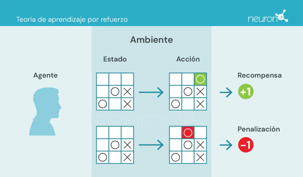
A classic reinforcement learning experiment is Skinner’s box, conducted by the American psychologist Burrhus Frederic Skinner in 1938. In this experiment, Skinner showed that rats could learn to press a lever to obtain food, using positive reinforcement as a means to shape behavior. 

The experiment consists of placing a rat in a box with a lever it can press, a food dispenser, and sometimes a light and a speaker. 

Each time the rat presses the lever, a food pellet is released into the dispenser. The food acts as positive reinforcement, a reward for pressing the lever. Over time, the rat will press the lever more frequently, demonstrating that it has learned the behavior through reinforcement.

This type of learning has served as the basis for machine learning algorithms, such as Q-learning, which allow machines to learn optimal behaviors autonomously through trial and error.

What is Q-learning?

Q-learning was introduced by Christopher Watkins in 1989 as a reinforcement learning algorithm. This algorithm allows an agent to learn the value of actions in a given state, continuously updating its knowledge through experience, much like the rat in Skinner’s box.

Unlike Pavlov’s experiments, where learning was based on simple associations, Q-learning uses a more complex method of trial and error. The agent explores various actions and updates a Q table that stores Q values, which represent the expected future rewards for taking the best action in a specific state.

Q-learning is applied in various areas, such as recommendation systems (like those used by Netflix or Spotify), in autonomous vehicles (such as drones or robots) and in resource optimization. We will now explore how this technology can be applied in neurorrehabilitation.

Q-learning and NeuronUP

One of the advantages of NeuronUP, is the ability to customize activities according to each user’s specific needs. However, customizing each activity can be tedious due to the large number of parameters to adjust. 

Q-learning allows this process to be automated, adjusting parameters based on the user’s performance in different activities. This ensures that exercises are challenging yet achievable, improving effectiveness and motivation during rehabilitation.

How does it work?

In this context, the agent, which could be compared to a user interacting with an activity, learns to make optimal decisions in different situations to successfully complete the activity. 

Q-learning allows the agent to experiment with various actions by interacting with its environment, receiving rewards or penalties, and updating a Q table that stores these Q values. These values represent the expected future rewards for taking the best action in a specific state. 

The Q-learning update rule is as follows:

\[Q(s,a) \leftarrow Q(s,a) + \alpha\bigl(r + \gamma \cdot \max_{a’}\bigl(Q(s’,a’)\bigr) – Q(s,a)\bigr)\]

Where:

𝛂 – is the learning rate.

r – is the reward received after taking action a from state s.

𝛄 – is the discount factor, which represents the importance of future rewards.

s’ – is the next state.

\(\max_{a’}\bigl(Q(s’,a’)\bigr)\) – is the maximum Q value for the next state s’.

Example of application in a NeuronUP activity

Let’s take the NeuronUP activity called “Mixed Images”, which works on skills such as planning, visuo-constructive praxis and spatial relationships. In this activity, the goal is to solve a puzzle that has been mixed and cut into pieces. 

The variables that define the difficulty of this activity are the board size (the number of rows and columns) as well as the disorder value of the pieces (low, medium, high or very high). 

To train the agent to solve the puzzle, a reward matrix was created based on the minimum number of moves required to solve it, defined by the following formula:

\[\mathrm{Min\_Attempts} \;=\;\left\lceil \frac{\mathrm{factor} * \mathrm{rows} * \mathrm{columns}}{5}\right\rceil,\quad \mathrm{factor}\in\{1,3,5,7\}\]

The factor variable depends on the disorder variable. Once the matrix was created, a Q-learning algorithm was applied to train the agent to solve the puzzle automatically. 

This integration includes:

• Retrieving the Q value: The function retrieves the Q value for a state-action pair from the Q table. If the state-action pair has not been trained before, it returns 0. This function looks up the expected reward when taking a specific action in a specific state.
• Updating the Q value: The function updates the Q value for a state-action pair based on the reward received and the maximum Q value of the next state. This function implements the Q-learning update rule mentioned earlier.
• Deciding which action to take: The function decides which action to take in a given state, using an epsilon-greedy strategy. This strategy balances exploration and exploitation: 
  • Exploration: Consists of selecting the best known action so far. With probability ε (exploration rate, a value between 0 and 1 that determines the likelihood of exploring new actions instead of exploiting known actions), a random action is chosen, allowing the agent to discover potentially better actions. 
  •  Exploitation: Consists of trying actions other than the best known ones to discover if they can offer better rewards in the future. With probability 1−ε, the agent selects the action with the highest Q value for the current state, using its learned knowledge: a’ = argmaxaQ(s,a). Where a’ is the action that maximizes the Q function in a given state s. This means that, given a state s, select the action a that has the highest Q value.

These functions work together to allow the Q-learning algorithm to develop an optimal strategy to solve the puzzle.

Preliminary analysis of the algorithm execution

The algorithm was applied to a 2×3 board puzzle with a difficulty factor of  1 (low), corresponding to a minimum number of attempts equal to 2. The algorithm was run on the same puzzle 20 times, applying the same mixing configuration each time and updating the Q table after each step. After 20 runs, the puzzle was shuffled into a different configuration and the process was repeated, resulting in a total of 2000 iterations. The initial parameter values were: 

• Reward for solving the puzzle: 100 points 
• Penalty for each move: -1 point

At each step, an additional reward or penalty was applied based on the number of correctly placed pieces, allowing the agent to understand its progress toward solving the puzzle. This was calculated using the formula:

\[W \times \bigl(N_{\mathrm{correct}}^i \;-\; N_{\mathrm{correct}}^{\,i-1}\bigr)\]

Where:

• W is the weight factor.
• \(N_{\mathrm{correct}}^{\,i}\) is the number of correct pieces after the move.
• \(N_{\mathrm{correct}}^{\,i-1}\) is the number of correct pieces before the move.

The graph below illustrates the number of moves required per iteration for the model to solve a 2×3 puzzle. At the beginning, the model requires a large number of moves, reflecting its lack of knowledge about how to solve the puzzle efficiently. However, as the Q-learning algorithm is trained, a downward trend in the number of moves is observed, suggesting that the model is learning to optimize its solving process.

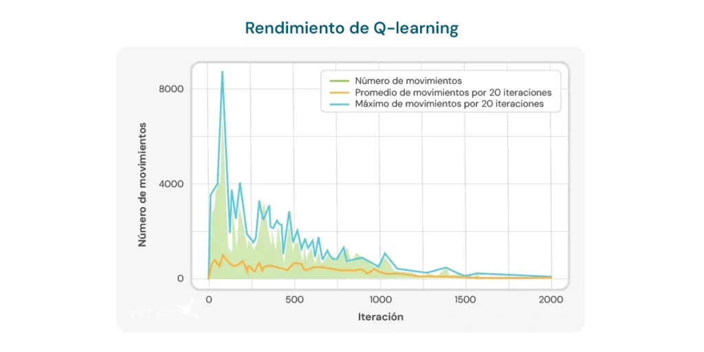
This trend is a positive indication of the algorithm’s potential to improve over time. However, several important limitations must be considered:

• Specific size of the Jigsaw Puzzle: The algorithm demonstrates effectiveness mainly on Jigsaw Puzzle of a specific size, such as the 2×3 board. Changing the size or complexity of the Jigsaw Puzzle can significantly reduce the algorithm’s performance.
• Computation time: When applying the algorithm to different or more complex configurations, the time required to perform the calculations and solve the Jigsaw Puzzle increases considerably. This limits its applicability in situations that require quick responses or in Jigsaw Puzzles with greater complexity.
• Number of moves still high: Despite the observed improvement, the number of moves required to solve the Jigsaw Puzzle remains relatively high, even after multiple iterations. In the final runs, the model requires an average of 8 to 10 moves, indicating that there is still room to improve learning efficiency.

These limitations underscore the need for further refinement of the algorithm, whether by adjusting learning parameters, improving the model structure or incorporating complementary techniques that enable more efficient learning and adaptability to different Jigsaw Puzzles. Despite these limitations, we should not forget the advantages that Q-learning offers in neurorrehabilitation, including:

• Dynamic personalization of activities: Q-learning is capable of automatically adjusting the parameters of therapeutic activities based on the individual user’s performance. This means that activities can be personalized in real time, ensuring that each user works at a level that is challenging but achievable. This is especially useful in neurorrehabilitation, where users’ abilities can vary significantly and change over time.
• An increase in motivation and engagement: As activities are constantly adapted to the user’s skill level, frustration from overly difficult tasks or boredom from overly simple tasks is avoided. This can significantly increase the user’s motivation and engagement with the rehabilitation program, which is crucial to achieving successful outcomes.
• Optimization of the learning process: By using Q-learning, the system can learn from the user’s previous interactions with activities, optimizing the learning and rehabilitation process. This allows exercises to be more effective, focusing on areas where the user needs more attention and reducing the time needed to reach therapeutic goals.
• Efficiency in clinical decision-making: Professionals can benefit from Q-learning by obtaining data-driven recommendations on how to adjust therapies. This facilitates more informed and precise clinical decisions, which in turn improves the quality of care provided to the user.
• Continuous improvement: Over time, the Q-learning-based system can improve its performance through the accumulation of user data and experience. This means that the more the system is used, the more effective it becomes in personalizing and optimizing exercises, thus offering a long-term advantage in the neurorrehabilitation process.

In conclusion, Q-learning has evolved from its roots in behavioral psychology to become a powerful tool in artificial intelligence and neurorrehabilitation. Its ability to autonomously adapt activities makes it a valuable resource to improve the effectiveness of rehabilitation therapies, although there are still challenges to overcome to fully optimize its application.

Bibliography

• Bermejo Fernández, E. (2017). Aplicación de algoritmos de reinforcement learning a juegos.
• Giró Gràcia, X., & Sancho Gil, J. M. (2022). La Inteligencia Artificial en la educación: Big data, cajas negras y solucionismo tecnológico.
• Meyn, S. (2023). Stability of Q-learning through design and optimism. arXiv preprint arXiv:2307.02632.
• Morinigo, C., & Fenner, I. (2021). Teorías del aprendizaje. Minerva Magazine of Science, 9(2), 1-36.
• M.-V. Aponte, G. Levieux y S. Natkin. (2009). Measuring the level of difficulty in single player video games. Entertainment Computing.
• P. Jan L., H. Bruce D., P. Shashank, B. Corinne J., & M. Andrew P. (2019). The Effect of Adaptive Difficulty Adjustment on the Effectiveness of a Game to Develop Executive Function Skills for Learners of Different Ages. Cognitive Development, pp. 49, 56–67.
• R. Anna N., Z. Matei & G. Thomas L. Optimally Designing Games for Cognitive Science Research. Computer Science Division and Department of Psychology, University of California, Berkeley.
• Toledo Sánchez, M. (2024). Aplicaciones del aprendizaje por refuerzo en videojuegos.

If you liked this article about the Q-learning, you will likely be interested in these NeuronUP articles:

“This article has been translated. Link to the original article in Spanish:”
Q-learning: Desde los experimentos de Pavlov a la neurorrehabilitación moderna